
Measuring a field into the simulator.
Our own rover’s simulated field was built before anyone measured the real one — rows at 3.05 m against a measured 2.30 m, a lane a third wider than the machine actually gets. This note is how the real field was measured out of the rover’s recordings and written back as a simulator stage, and the main factors affecting reconstruction quality. It assumes a reader who works with ROS 2 and a simulator.
The simulated rows were 33% wider than the real ones.
Our initial simulation scene was assembled before the real environment had been measured. Our Isaac Sim field had rows 3.05 m apart. The rover’s LiDAR says the real rows sit 2.30 m apart — so anything that held a line in that model had been handed roughly a third more lane than the field gives it, and every line-holding result from the twin was optimistic as a consequence.
Rather than redraw the scene more carefully, we generated it from measurements. Selected field recordings supplied the sensor data used for this reconstruction. The pipeline goes recording → measured geometry → a text USD stage that loads, collides and renders. When the rows grow next season, the stage can be regenerated from new recordings and diffed against this one.
Updated field scene: two camera views
Updated field scene with detailed blueberry models. Scripted motion illustrates the scene; the measurements discussed here come from the earlier comparison runs.
Earlier camera-based reconstruction
This earlier reconstruction combines LiDAR-derived collision geometry with camera-based appearance. It is separate from the authored bush models above; detail is soft and useful viewpoints remain close to the capture path.
Row spacing is measured inside a single sweep.
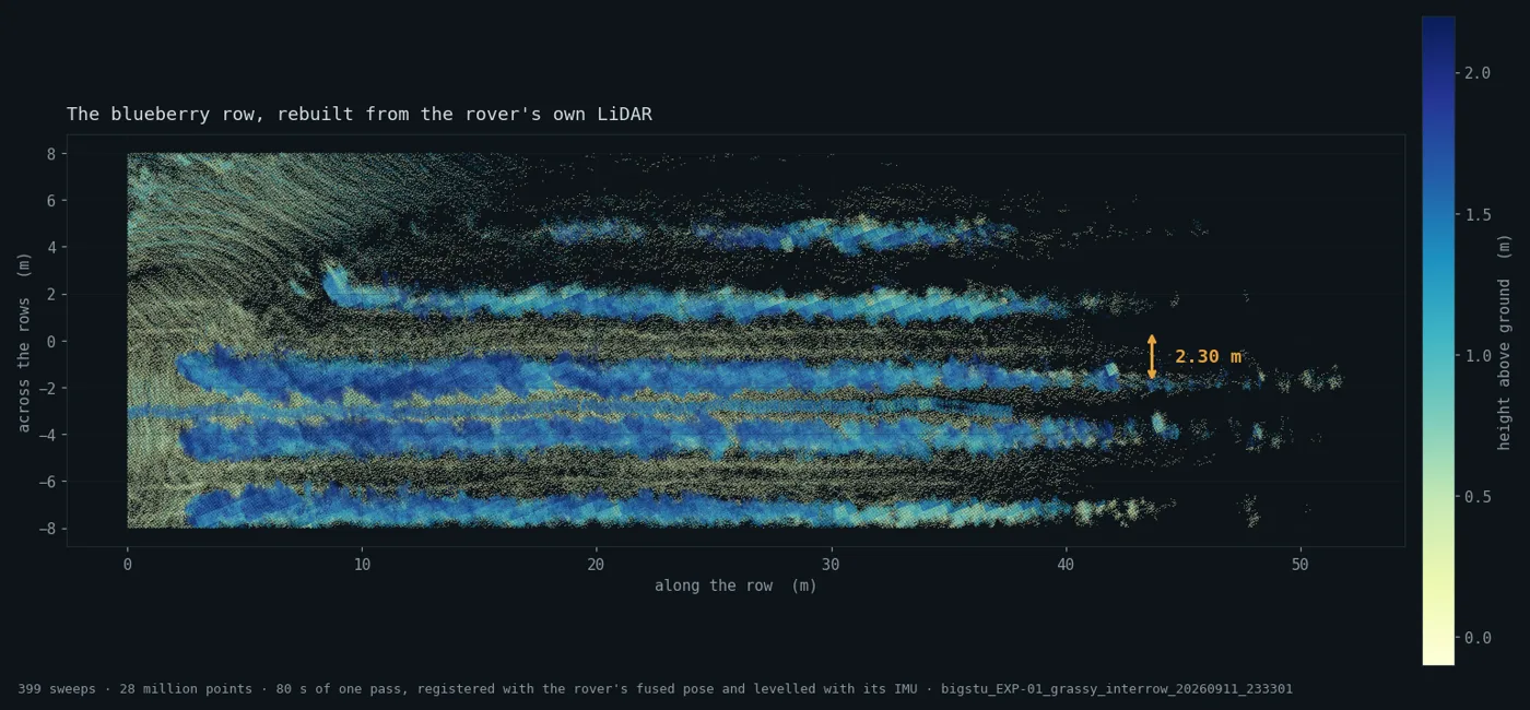
Row spacing is measured inside a single 100 ms LiDAR sweep, not accumulated across the run. A 40-beam LiDAR standing in a lane sees several rows to each side at once, so the spacing is visible within one sweep, where odometry drift cannot affect it.
The pipeline keeps the two kinds of measurement separate. The per-sweep spacing avoids accumulated odometry drift, so it is what goes into the stage. The registered cloud — every sweep placed in the run’s odom frame — carries whatever the EKF drifted, and exists to recover terrain and make pictures. Its own row detector is constrained by the per-sweep spacing, precisely because it is the less reliable of the two: a row smeared by a few centimetres grows a twin peak, and an unconstrained peak finder then reports half the true spacing.
Surveyed across six recordings from four field sessions — 24 sweeps sampled from each — every pair of neighbouring rows the LiDAR resolved:
| Recording | Row pairs | Median spacing | Canopy top |
|---|---|---|---|
| Session D | 27 | 2.300 m | 1.90 m |
| Session C · run 1 | 22 | 2.300 m | 1.92 m |
| Session C · run 2 | 28 | 2.300 m | 1.89 m |
| Session B · run 1 | 31 | 2.200 m | 1.89 m |
| Session B · run 2 | 27 | 2.300 m | 1.89 m |
| Session A | 21 | 2.200 m | 1.93 m |
| Pooled | 156 | 2.300 m IQR 2.19–2.50 | ~1.90 m |
Everything runs under plain python3 with a hand-written MCAP reader and CDR decoders — no ROS install, no container, no rover — and the measurement scripts carry --self-test flags that assert their own maths against synthetic input. The stage is emitted as text USDA rather than through the USD Python bindings, so it can be generated on any machine and diffed when the field is measured again.
Five factors affecting reconstruction quality.
Account for the IMU mounting frame when correcting terrain tilt.
The extended Kalman filter (EKF) uses a planar motion model and does not estimate roll or pitch. On uneven terrain, registering LiDAR sweeps without correcting these angles introduces vertical error that increases with distance. A 2° tilt produces approximately 0.70 m of vertical displacement at a range of 20 m.
The inertial measurement unit (IMU) reports orientation in its mounted sensor frame. Interpreting those angles directly as vehicle attitude introduced an apparent roll of −101°. In the resulting reconstruction, estimated terrain relief reached 38 m and only one of eight rows was detected.
The revised method estimates the sensor’s reference orientation from the median world-up direction over each recording window. Individual sweeps are levelled relative to that reference, while yaw remains supplied by the EKF. This approach assumes that the window provides a suitable reference orientation; a sensor remount requires verification. In Session D, the estimated tilt had a median of 1.65° and a maximum of 7.36°.
Ground estimates depend on visibility beneath the canopy.
Ground height was initially estimated from the fifth percentile of LiDAR returns in each 0.5 m cell. This statistic represents ground level only where the sensor observes the ground. Vegetation and other structures can bias it upward, particularly beneath dense canopy.
The analysis was restricted to a 12 m corridor around the recorded path. Within that corridor, the reported 0.50 m RMS variation included grass, canopy returns and registration error, so it could not be interpreted directly as terrain relief. The stage retains the estimated 0.40° slope across 8,519 cells and limits local relief to ±0.25 m. This limit is a modelling constraint, not a measured bound on the field’s surface. Applications sensitive to ground relief require additional ground measurements.
Distinguish cumulative heading variation from net heading change.
The initial selection method ranked recording windows by cumulative yaw variation. Repeated steering corrections of approximately ±10° accumulated to 261° over an 80-second pass, despite the rover generally following the row. This metric therefore penalised local corrections without reliably identifying unsuitable passes.
Filtering by net heading change selected a 56.8 m pass with a 0.1° change between its start and end. Net change is useful for screening candidate windows, but does not independently establish that the rover remained within one row.
Validate collision volume as well as the measured silhouette.
The first row colliders were extruded directly from canopy silhouettes. Where the measured canopy top was nearly level, the extrusion produced a surface at approximately 1.8 m with no vertical extent. Ground contact still worked, so a drive-through could appear plausible even though the rows did not provide the intended collision boundaries.
The revised construction extends the silhouette to ground level at its outer boundary. A regression check uses a deliberately flat silhouette to verify that the resulting collider retains vertical extent and reaches the ground.
Evaluate spatial detail alongside image similarity.
The appearance reconstruction uses 739 forward-camera frames, with camera poses derived from the EKF and the recorded sensor transforms. LiDAR returns provide the initial geometry. This reduces reliance on structure-from-motion in a scene containing many similar bushes.
Peak signal-to-noise ratio (PSNR) alone did not distinguish useful reconstruction from smooth, low-detail output. One run scored 16.82 while retaining almost no visible structure. Evaluation therefore also uses a sharpness ratio: the rendered image’s Laplacian variance divided by that of the reference image. This measures relative image detail; it is not a direct measure of geometric accuracy.
| Run | Frames | Gaussians | PSNR | Sharpness |
|---|---|---|---|---|
| gsplat, pose optimisation on | 739 | 2.5M | 12.86 | 0.0% — misaligned |
| 3DGUT, MCMC densification | 739 | 2.5M | 16.82 | 0.1% — low detail |
| 3DGUT, default strategy | 739 | 710k | 18.00 | 3.7% |
| 3DGUT, densify ×2 | 739 | 949k | 17.82 | 3.8% |
The experiments identified separate alignment and initialisation issues. Pose optimisation displaced the reconstruction from the measured reference frame. With the tested MCMC densification configuration, assumptions suited to a sparse structure-from-motion cloud produced millimetre-scale Gaussians from approximately 500,000 LiDAR points in a 30 m corridor; subsequent perturbations dispersed them over approximately ±750 m.
The default 3DGUT strategy improved alignment and detail. Increasing the Gaussian count from 710,000 to 949,000—approximately 34%—changed the sharpness ratio only from 3.7% to 3.8%, while PSNR decreased from 18.00 to 17.82. Increasing model density alone therefore provided little improvement in these runs.
The input images had a Laplacian variance of approximately 1,200, indicating substantially more image detail than the reconstructions. Limited lateral camera displacement is a plausible constraint: a predominantly forward pass provides fewer complementary viewpoints than an offset capture. A second pass with lateral separation is a proposed next experiment. Independently enhancing each input image could introduce inconsistent or invented detail, so it would require separate evaluation before use in a measurement-based workflow.
Verify scene alignment, collision behaviour and motion response separately.
The verification procedure opens the stage in Isaac Sim, checks collision configuration, advances the physics simulation and renders from lane height. A simulated drive-through provides an additional check that the separately generated appearance and collision geometry remain aligned. This exposed a training configuration that normalised the scene’s scale and displaced it from the intended metric frame—an issue not identified by image-quality metrics alone.
These checks establish aspects of scene assembly and ground contact. They do not establish that the simulated robot reproduces the physical vehicle’s steering response.
Building a simulation scene of a real environment?
Discuss your environment and sensors on a free twenty-minute call. We review the available recordings or drawings before quoting any build or site measurements.